Visualizing a Live C++ Model in Python
C++ is good at some things, and Python is good at others
04/16/2023
20 Minutes to Read
[c++ python dashboarding visualization simulation model panel holoviews pybind11 C++ lets us write fast code, but Python lets us better understand our model.
Python is just too good at many things, and of the many things it is good at, it is very good at analyzing and visualizing data. Analyzing and visualizing data are usually very exploratory processes, and so that code is changing frequently. Changing Python is much easier than changing C++, and so it fits very well into that workflow.
For example, if we model an n-body system (perhaps like the one we breezed by here), then we very clearly have a reason to want to code in C++. But we also want to analyze the model, visualize its data, or maybe script some custom control over the model. We are going to start with that code and pull it apart into a handful of pieces that make using it in Python easy.
We should also note now that we do not want to run our C++ program as a subprocess in Python - this offers the least amount of flexibility and forces us to handle data through pipes or disk IO. We want Python and C++ communicating directly with one another!
One final note before we begin - visualizing models like this has been a true game-changer in the scientific computing course that I teach. I have been adding live dashboards to almost all of our work to help give students better context over what they are coding and the feedback so far has been overwhelmingly positive!
Updating our Code
Let’s first just take a look at the standalone C++ model that we want to use from Python. In case you are just catching up, this code implements a brute-force n-body simulation. We have many particles all interacting gravitationally with each other:
// main.cpp
#include <cmath>
#include <fstream>
#include <random>
#include <vector>
#include <fmt/format.h>
#include <fmt/ostream.h>

constexpr double GRAVITY = 6.6743e-11;  // Newton's Gravitational Constant

struct Particle {
    double x = 0.0;
    double y = 0.0;
    double vx = 0.0;
    double vy = 0.0;
    double ax = 0.0;
    double ay = 0.0;
    double mass = 5.0e6;

    void integrate(const double dt) {
        vx += ax * dt;
        vy += ay * dt;
        x += vx * dt;
        y += vy * dt;
        ax = 0.0;
        ay = 0.0;
    }

    void add_force(const Particle &other) {
        double dx = other.x - x;
        double dy = other.y - y;
        double distance = std::hypot(dx, dy);
        double direction = std::atan2(dy, dx);
        double force = GRAVITY * other.mass / (distance * distance);
        ax += force * std::cos(direction);
        ay += force * std::sin(direction);
    }
};

int main() {
    std::mt19937 eng;
    std::uniform_real_distribution<double> dis(-50.0, 50.0);

    int num_particles = 1000;
    std::vector<Particle> particles;
    particles.reserve(num_particles);
    for (auto i = 0; i < num_particles-1; ++i) {
        particles.emplace_back(dis(eng), dis(eng));
    }
    particles.emplace_back(0, 0, 0, 0, 0, 0, 1e12);

    double time_delta = 0.1;
    double simulation_time = 0.0;
    double max_simulation_time = 50.0;

    std::ofstream csvfile("particles.csv");
    while (simulation_time < max_simulation_time) {
        for (auto &p1 : particles) {
            for (const auto &p2 : particles) {
                if (&p1 == &p2) continue;
                p1.add_force(p2);
            }
        }
        for (auto &p1 : particles) {
            p1.integrate(time_delta);
            fmt::print(csvfile, "{:.8f},{:.8f},{:.8f},{:.8f}\n", simulation_time, p1.mass, p1.x, p1.y);
        }
        simulation_time += time_delta;
    }
}
There are a few issues with how our program currently works that make using it as a Python module difficult. We are going to do the following:
- Move the
Particleclass to its own header (just for simplicity) - Create a new class,
ParticleSystem, that has its own header- this class should capture the initialization and update logic of the model, but not necessarily the flow (e.g. the while-loop).
// particle_system.h
#pragma once

#include <random>
#include <vector>
#include "particle.h"

struct ParticleSystem {
    ParticleSystem(const int num_particles, const double bounds, const int seed=1337) {
        std::mt19937 eng(seed);
        std::uniform_real_distribution<double> dis(-bounds, bounds);
        particles.reserve(num_particles);
        for (auto i = 0; i < num_particles-1; ++i) {
            particles.emplace_back(dis(eng), dis(eng));
        }
        particles.emplace_back(0, 0, 0, 0, 0, 0, 1e12);
    }

    void update(const double time_delta) {
        for (auto &p1 : particles) {
            for (const auto &p2 : particles) {
                if (&p1 == &p2) continue;
                p1.add_force(p2);
            }
        }
        for (auto &p1 : particles) {
            p1.integrate(time_delta);
        }
    }

    std::vector<Particle> particles;
};
It is important to note that this class does not capture the while-loop! While we could have done so, the while-loop is less a part of the model and more a part of the executor of the model. It represents the flow of time, which users of the model should control. What this class does allow us to do is create a set of particles, and then advance their state through time.
With our ParticleSystem class now ready we can expose it to Python using pybind11!
pybind11
pybind11 is…
... is a lightweight header-only library that exposes C++ types in Python and vice versa, mainly to create Python bindings of existing C++ code. Its goals and syntax are similar to the excellent Boost.Python library by David Abrahams: to minimize boilerplate code in traditional extension modules by inferring type information using compile-time introspection.
What this allows us to do is wrap our C++ code using a few minimal constructs and patterns defined by pybind11, and then we can build that wrapper into a library that Python can import. We want to expose our newly made ParticleSystem to Python; to do so we need to tell pybind11 what members of the class are to be made available. We will need to expose the constructor, the update method, and the particles vector. We also want to open up the Particle class so that we can access the kinematics through its x, y, vx, and vy members.
Here is our heavily commented pybind11 wrapper for our model:
// particle_model.cpp
#include <pybind11/pybind11.h>  // include pybind11
#include <pybind11/stl.h>       // needed when binding STL types
namespace py = pybind11;

#include "particle_system.h"

// this macro names our Python module "ParticleModel" and we can use
// m to reference the module in the following block of code.
PYBIND11_MODULE(ParticleModel, m) {
    // define a Python class named "ParticleSystem" from our C++ ParticleSystem class
    // - expose the constructor; we give it a template specifying the signature
    //   of the inputs
    // - expose the version of our constructor using the default value for the random seed
    // - expose the update method, matching it to the update method of our class
    // - expose the particles vector as both readable and writable
    py::class_<ParticleSystem>(m, "ParticleSystem")
        .def(py::init<const int, const double, const int>())
        .def(py::init<const int, const double>())
        .def("update", &ParticleSystem::update)
        .def_readwrite("particles", &ParticleSystem::particles);

    // define a Python class named "Particle" from our C++ Particle class
    // - expose the x position as both readable and writable
    // - expose the y position as both readable and writable
    // - expose the vx velocity as both readable and writable
    // - expose the vy velocity as both readable and writable
    py::class_<Particle>(m, "Particle")
        .def_readwrite("x", &Particle::x)
        .def_readwrite("y", &Particle::y)
        .def_readwrite("vx", &Particle::vx)
        .def_readwrite("vy", &Particle::vy);
}
And that is it! Simple, right? While I am not going to cover compilers, versions, and installation of all of these things (follow the docs!), assuming you have a typical environment then all we need to do to build this into a module usable by Python is:
g++-12 -std=c++20 -O3 -shared -fPIC $(python3 -m pybind11 --includes) particle_model.cpp -o ParticleModel$(python3-config --extension-suffix)
We are using g++-12 as before, but we have a few additions here.
-std=c++20- while ourpybind11code does not require C++20, our model code does-O3- enable compiler optimizations heavily geared towards performance-shared- we are building a shard-object rather than an executable, so we need to tell it to link as such-fPIC- because we are building a shared-object we need to ensure the compiled binary can be dynamically loaded in memory properly$(python3 -m pybind11 --includes)- assuming we have installedpybind11into our Python environment, we can call into it to get the paths to its headersparticle_model.cpp- the binding code we wrote above-o ParticleModel$(python3-config --extension-suffix)- output the shared-object with the proper suffix
On my system this yields a file that looks like this:
ParticleModel.cpython-310-x86_64-linux-gnu.so
In Python we can now import and use this module! From the directory containing the new share-object:
from ParticleModel import ParticleSystem
model = ParticleSystem(100, 50)  # create a system of 100 particles in the range [-50, 50] in both the x and y axes
for i in range(10):  # update the system 10 times
    model.update(0.1)
    for particle in model.particles:
        print(f'<{particle.x:.2f}, {particle.y:.2f}>')
Perfect! Or well, sort of… seeing raw positional data is not very useful… so lets visualize it!
Visualizing Our C++ Model
The little snippet above shows us that we can now import and use our model in a Python context, but what can we do with this now? The answer is a lot! Python is very well suited to visualize data, and so we are going to use it to run and visualize our particles in a live dashboard. We are going to use Python library Panel to assemble the dashboard and HoloViews to produce the visualizations! For brevity we are going to start with a very simple dashboard. In a future post we will dive deeper and make something much more detailed.
There are some fairly complex things in this “simple” dashboard, and it may look like a lot, but it is not too bad once we step through it and understand what it is doing (hopefully). Here is the general breakdown of how we set everything up, followed by the (heavily commented code).
Our dashboard is going to work by creating an instance of our model and then updating and visualizing that model repeatedly. We also want to provide some ability to configure the model using a few widgets; for now we will control the number of particles, the bounds to generate the particles within, and the time delta for updating the model.
To start we need to define callbacks to handle a few different events:
update_model: this callback should update the state of the model; we will trigger this often and automaticallyvisualize_model: this callback should return a visualization of the current model state; this will be triggered byupdate_modelplay: this should trigger the simulation to start playing; this will be triggered by a buttonreset: this should reset the model state and visualization; this will be triggered by a button
We will also use a few global variables:
model: instance of our C++ modelentity_pipe: an object to help stream data from the model to the visualizationperiodic_callback: an object that manages a continuous periodic callback
And finally we will define a few widgets:
play_button: start/stop the simulationreset_button: reset the simulationnum_particles_slider: control the number of particles simulatedbounds_slider: control the bounds within which particles are generatedtime_delta_slider: control the size of the time step when updating the model
Once we have all of these defined, we can pack the widgets and visualization into a layout. The general flow is straightforward - we have an instance of our model and a function that updates that instance (basically our while-loop from our initial code!). Whenever we update the model we stream its state to a visualization. - this gives us a live animation of the model’s state.
"""main.py

Defines a Panel dashboard for visualizing the native ParticleModel extension
"""

import holoviews as hv  # for plotting
import numpy as np      # for some data manipulations
import pandas as pd     # for setting up our data
import panel as pn      # for dashboarding
import param as pr      # for a typehint
from holoviews.streams import Pipe        # for continuously streaming data to the plot

from ParticleModel import ParticleSystem  # our C++ model!

def update_model() -> None:
    """Callback that is executed by periodic callback managed by the dashboard.

    Update the model by a single step using the time delta. Once updated the
    model data is packed into a dataframe and sent through the pipe.
    """
    model.update(time_delta_slider.value)
    particle_data = pd.DataFrame([[particle.x, particle.y] for particle in model.particles], columns=['x','y'])
    entity_pipe.send(particle_data)

def visualize_model(data: pd.DataFrame) -> hv.Points:
    """Callback that is executed whenever data is streamed through the pipe.

    From the model state (as sent from update_model) a scatter plot is created,
    plotting the x-position against the y-position, giving a bird's-eye view of
    the simulation.

    We also set the dimensions of the plot and the dimensions of the data, as
    well as enable the grid.

    Arguments:
        data: single state of the simulation

    Returns:
        HoloViews Points element; a scatter plot of the model state
    """
    return hv.Points(data, kdims=['x', 'y']).opts(
        height=640,
        width=640,
        xlim=(-bounds_slider.value, bounds_slider.value),
        ylim=(-bounds_slider.value, bounds_slider.value),
        show_grid=True
    )

def play(event: pr.parameterized.Event) -> None:
    """Callback to play the simulation.

    Configures a periodic callback to execute our update_model callback
    approximately 30 frames-per-second. If the callback is already scheduled
    then disable it. Also changes the button name to indicate the state.

    Arguments:
        event: the click event that triggered the callback
    """
    global periodic_callback
    if periodic_callback is None or not periodic_callback.running:
        play_button.name = 'Stop'
        # set the periodic to call our run_model callback at 30 frames per second
        periodic_callback = pn.state.add_periodic_callback(update_model, period=1000//30)
    elif periodic_callback.running:
        play_button.name = 'Play'
        periodic_callback.stop()

def reset(event: pr.parameterized.Event | None) -> None:
    """Callback to reset the simulation.

    Stops periodic callback if active; remove the period callback, recreate the
    model, and stream the initial model state through the pipe.

    Arguments:
        event: the click event (or None when initialized) that triggered the
        callback
    """
    global model, periodic_callback
    if periodic_callback is not None and periodic_callback.running:
        play_button.name = 'Play'
        periodic_callback.stop()
    periodic_callback = None
    model = ParticleSystem(num_particles_slider.value, bounds_slider.value)
    particle_data = pd.DataFrame([[particle.x, particle.y] for particle in model.particles], columns=['x','y'])
    entity_pipe.send(particle_data)

# create a global for the model
model = None

# we use a pipe so that we can stream data from an asynchronous periodic callback
entity_pipe = Pipe(data=[])

# create a global periodic callback - with it being global and persisted we can
# start and stop it at will
periodic_callback = None

# play button, with the play callback attached to the on-click event of the button
play_button = pn.widgets.Button(name='Play')
play_button.on_click(play)

# reset button, with the reset callback attached to the on-click event of the button
reset_button = pn.widgets.Button(name='Reset')
reset_button.on_click(reset)

# input sliders for various options
num_particles_slider = pn.widgets.FloatSlider(name='Number of Particles', start=1, end=1000, step=1, value=100)
bounds_slider = pn.widgets.FloatSlider(name='Bounds', start=25, end=2500, value=100, step=25)
time_delta_slider = pn.widgets.FloatSlider(name='Time Delta (s)', start=0.1, end=1.0, value=0.1, step=0.1)

# upon loading the dashboard, reset the model and view
pn.state.onload(lambda: reset(None))

# assemble everything in one of the built-in templates
pn.template.MaterialTemplate(
    site="Particle Model ",
    main=[
        # this is important! the DynamicMap ties the plotting callback to the pipe!
        hv.DynamicMap(visualize_model, streams=[entity_pipe])
    ],
    sidebar=[
        num_particles_slider,
        bounds_slider,
        time_delta_slider,
        play_button,
        reset_button
    ]
).servable() # set the template as servable so that we can... serve it!
This heavily commented code is ~125 lines long, but really it is closer to maybe 70 lines if we strip it down. We can run the dashboard by saving this main.py to the same directory that contains our compiled C++ model, and then by running the following command:
panel serve main.py
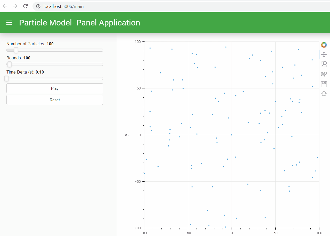
This will launch a local webserver that you can access in your browser. You should see something like this:
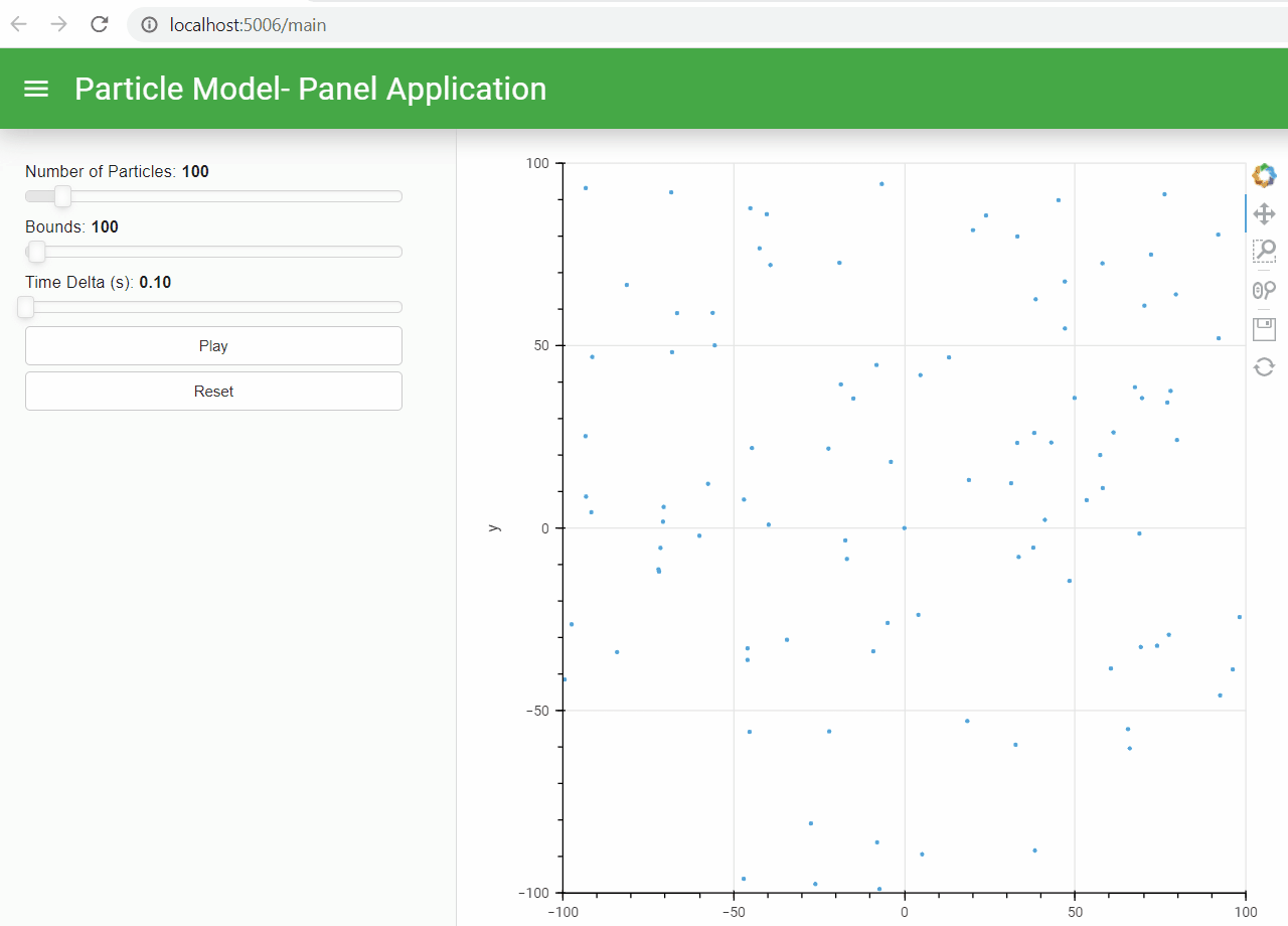
The particles are pulled towards the center because our model creates a very heavy particle at the origin that overwhelmingly attracts the other particles. When two particles get arbitrarily close the force due to gravity approaches infinity, and because we are not modeling collisions, the particles will just shoot out of orbit.
We can do much more from here, but for now we are just going to update the initial state of the model from Python to give it a twist! Let’s change our reset function by adding the following code right before building the dataframe:
    for particle in model.particles:
        r = np.hypot(particle.x, particle.y)
        if r > 1.0e-8:
            particle.vx = -particle.y / r
            particle.vy = particle.x / r
This code updates the particles within the model by sending them on a small counter-clockwise trajectory based on the quadrant they are in. This gives us a rather satisfying swirling motion!
Depending on your machine, simulating 1000 particles may be a bit clunky (even in the gifs above you can see a little bit of stuttering) - the little bits of choppiness in the animations are due to the model updates taking more than ~33 milliseconds. We are using the brute-force method for updating the model, but we could achieve better performance using a Barnes-Hut Approximation, or even multithreading (true multithreading from C++!), or any number of other solutions. If we had written this model in Python we would likely be dealing with even worse performance issues (assuming we are not properly using NumPy and/or Numba!).
Final Notes
To recap - we started with a standalone C++ program that generated CSVs. Then we pulled the code apart to isolate the core model and logic, and wrapped that core model using pybind11 to make it usable from within Python. And finally we wrote a dashboard to instantiate, update, and visualize our model using Panel and HoloViews. The final set of code used in this post can be found here.
We can go a lot further with improving both our model (to make it more configurable, more performant) and our dashboard, but this post was sort of already blowing up a good bit. In future posts we will cover some optimizations for the model, and in another post we will add even more to our dashboard to update both its functionality and its aesthetics.
In the meantime check out the projects used to build this, there are endless possibilities! With all of these tools we can create some astoundingly powerful simulations and visualizations, all we need to do is just throw some code together and these tools take care of the rest!